New Mexico Tech
Earth and Environmental Science
ERTH 471 / GEOP 572 - Geodetic Methods
Lab 11: Modeling: Timeseries Fitting
UNAVCO bumper sticker
Note that you DON'T have to work on redoubt today!
Introduction
Last week you learned about CATS and how you can estimate certain parameters in a timeseres using this tool. Today, you will do this yourself! I will give you 3 component data and you will invert for parameters of several linear models that we expect in the time series data.
1. Say Hi to FICT
FICT is a fictitious GPS site near some plate interface. Its long term trend looks like travel to the SSE and during its time it experienced an earthquake on day 413, which set it back to the NNW. There's quite some action in the seasonality, too. This is what the time series looks like in 3 components:
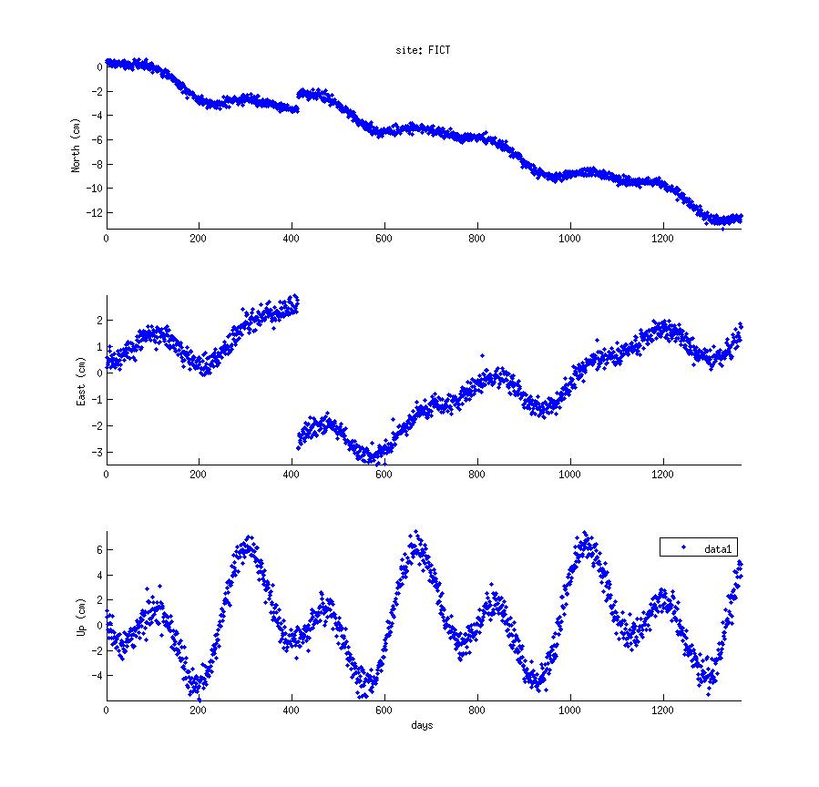
I'd recommend you start out with recreating this plot. You can download the data for Matlab here.
2. Background
I created these timeseries using a model that is a scaled superposition of:
- y-offset
- gradient (velocity)
- annual sine and cosine
- semiannual sine and cosine
- heaviside function with offset at day 413.
h_vec = [-1 * ones(413, 1); ones(total_days-413+1,1)];
where total_days is the length of the timeseries in one component. This gives you a function that is zero until day 413 and
after day 413. (in Matlab heaviside(h_vec)).
Your first task: Write the model equation for 1 component. The equation should contain 7 coefficients.
We use the same model (equation) for all three components, but as you can see in the time series, the coefficient values will come out differently. This is easily justified: the same physics affect one site, but they act differently on it depending on the direction.
3. The Fitting - Part 1
You now have an understanding of the model and you are aware that you need to find 7 model parameters for each component. How to go about this? Yes, let's try least-squares!
Recall that:
d = G * m
At this stage you can make a huge mistake: trying to solve the problem for all components at once. Don't do that!
How about we try to figure out the fit for the North component first and then we expand in the other directions? And even
better - start model component by model component!
To begin with: Your d will be dN as it is in the mat file. The m - model
parameters are what you want. G will have model-parameter many columns, and data point many rows. Try setting up
G for a linear fit first:
d = a + b*x
How many columns has G, what are the values in the columns?
Now solve the inverse problem:
m = G \ d
The backslash operator is probably the most powerful operator in Matlab, which will give you the least-squares solution to your
problem. Other possibilities are:
    m = inv(G) * d
    m = pinv(G) * d
    m = inv(G'*G) * G' * d
	...
Your model vector should now contain 2 parameters, a_m, b_m. Modify your plotting routine such that
d = a_m + b_m * x
is plotted on top of your North time series (should look similar to the black line
in the upper panel of the figure below). What are the units of a,b? Convert
the velocity (b) to cm/year.
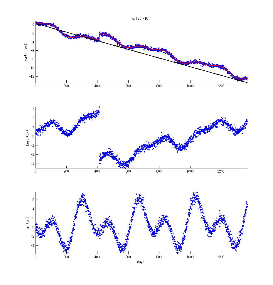
Once you've got G set up for two of your model components, the expansion to the
5 others should be straightforward: add the scaling factors to m and the (unit) functions
(i.e. unscaled functions) as columns into G. Their order won't matter, as long as
you keep the order of the respective scaling factors the same. Plot the model over the time series
and it should look like the red line in the upper panel of the figure above (You get that by solving
the forward model, i.e. the equation you've written out at the beginning.)
4. The Fitting - Part 2
You are 2 critical steps away from being able to fit all three timeseries using 1 least squares inversion. Even though I am not giving any covariances here to properly weight the data, recall that the full least-squares solution is:
m = (G'WG)^(-1) * G'Wd
Where W could be the inverse of the covariance matrix. Once you think about covariances you should realize
that you'd need to invert for all parameters that characterize the timeseries in your three components at
the same time.
With that in the back of your minds you want to set up 1 data vector and 1 design matrix to get 1 model vector. The trick is to think in subsets! Create 1 long column vector containing all your data. The first third will be, maybe, the north component; the middle third will be the east component and the last third could be the vertical component.
This idea maps directly into your result / model vector: The first 7 components will be the ones describing the north time series, the middle 7 components will describe the east time series, and the last 7 components will characterize the vertical.
Understanding and doing this, was the first critical step. The second step involves the proper expansion of
your design matrix G. You will need to add blocks of zeros so that you end up with something
like this:
         [ GN  0  0 ]
     G = [  0 GE  0 ]
         [  0  0 GU ]
where GN is exactly the design matrix you created in section 3. In fact, GN = GE = GU. And
each zero represents a matrix of size of GN filled with zeros.
Create a plot like this one:
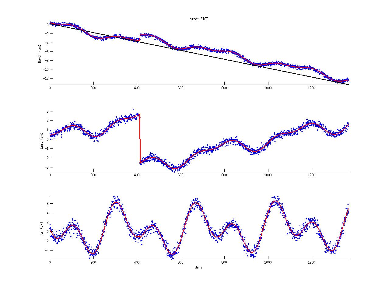
What is the static offset at day 413 in all 3 components? How does this compare to the "plate motion" or long term velocity? What are amplitude and azimuth of the horizontal motion for this event? What is the annual sine and cosine amplitude in the vertical component? Is this overall a convincing time series, or do you see any issues?
Deliverables: (submit via canvas!)
- Your script that creates the plots
- The plot with the fits as jpg
- Answers to questions in bold in separate document.